Alignment
Working directory
Open your terminal, and go to your working directory,
cd /mnt/albasj/analysis/username
and create the following directory structure:
mkdir stats
mkdir alignment
mkdir variant_calling
FASTQ
The data we will be using is a subset of specific regions of chromosome X in a FASTQ format. FASTQ format is a text-based format for storing both a biological sequence and its corresponding quality scores.
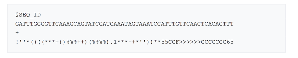
A FASTQ file normally uses four lines per sequence: 1) Begins with a ‘@’ and is followed by a sequence identifier 2) Is the raw sequence letters 3) Begins with a ‘+’ character 4) Encodes the quality values for the sequence in Line 2
You can visualize the FASTQ file typing:
less -S /mnt/albasj/data/nanopore/fastq/child.nanopore.ROI.fastq
How many reads do we have?
awk '{s++}END{print s/4}' /mnt/albasj/data/nanopore/fastq/child.nanopore.ROI.fastq
Reads QC
First we will get the read length for each read:
awk '{if(NR%4==2) print length($1)}' /mnt/albasj/data/nanopore/fastq/child.nanopore.ROI.fastq > stats/read_length.txt
And look at the read length distribution. For that, you can start R from the command-line:
R
and then, type the following:
library(ggplot2)
readLength <- read.table("stats/read_length.txt", header=FALSE, col.names = "length")
ggplot(data=readLength, aes(length)) + geom_histogram()
Hint: for quitting R, just type, quit()
Alignment
The standard format for aligned sequence data is SAM (Sequence Alignment Map).
SAM files have a header that contains information on alignment and contigs used, and the aligned reads:
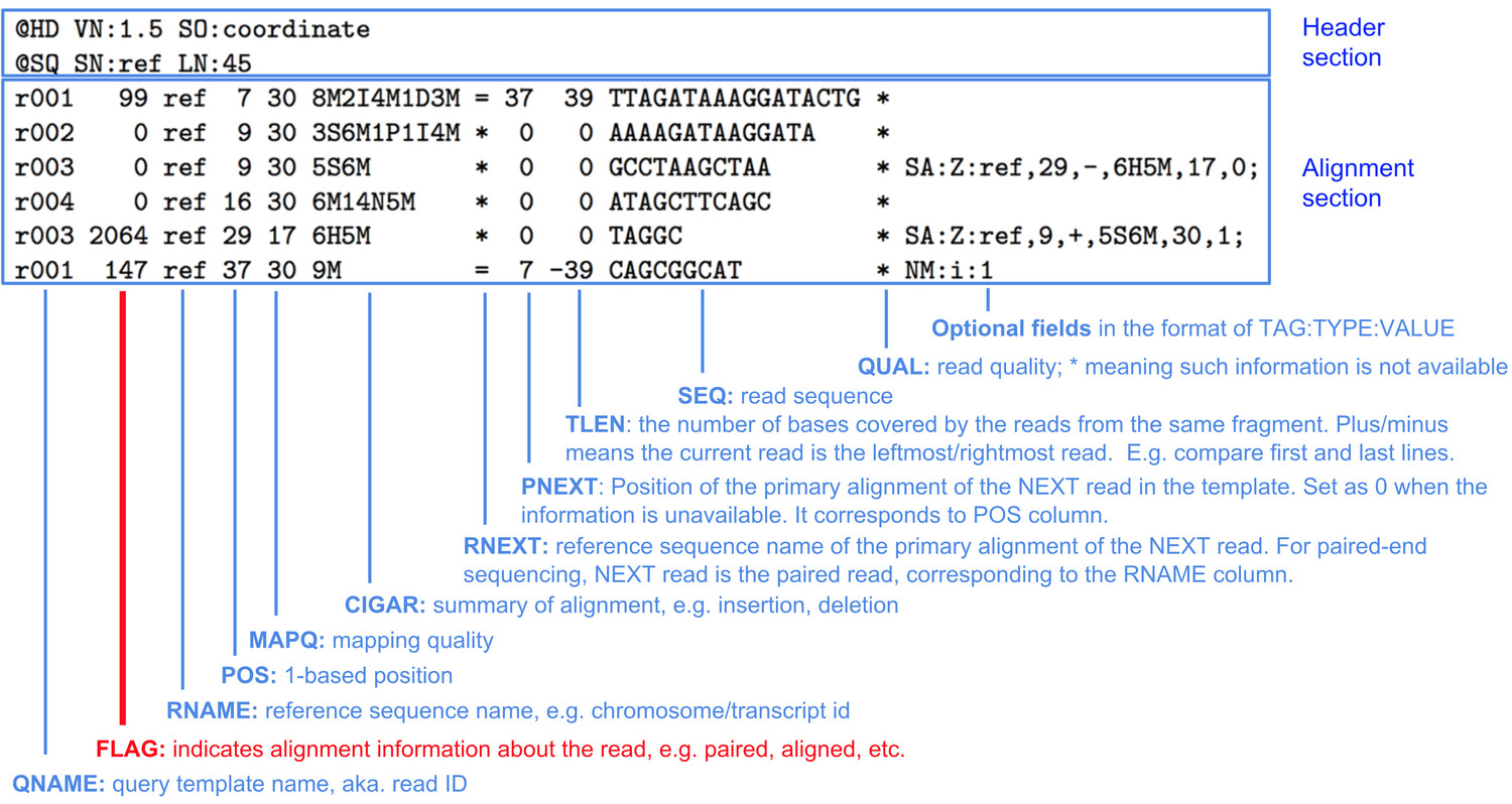
But because SAM files can be large, they are usually stored in the compressed version of them, BAM files.
Multiple algorithms have been developed to align long reads to a genome of reference. Some examples are:
- Graphmap: http://github.com/isovic/graphmap
- bwa mem -x l ont2d: http://github.com/lh3/bwa
- LAST: http://last.cbrc.jp
- NGMLR: http://github.com/philres/ngmlr
- minimap2: http://github.com/lh3/minimap2
Here we will use NGMLR. First we will map the reads to the genome of reference (GRCh37)
ngmlr -r /mnt/albasj/data/reference/GRCh37/Homo_sapiens.GRCh37.75.dna.fasta \
 -q /mnt/albasj/data/nanopore/fastq/child.nanopore.ROI.fastq \
 -o alignment/child.nanopore.ROI.sam
and convert the SAM output to BAM format.
samtools view alignment/child.nanopore.ROI.sam \
 -O BAM \
 -o alignment/child.nanopore.ROI.bam
Then, we will sort it by mapping coordinate and save it as BAM.
samtools sort -o alignment/child.nanopore.ROI.sort.bam alignment/child.nanopore.ROI.bam
Finally we will index the BAM file to run samtools subtools later.
samtools index alignment/child.nanopore.ROI.sort.bam
To visualise the BAM file:
samtools view -h alignment/child.nanopore.ROI.sort.bam | less -S
Alignment QC
As a first QC, we can run samtools stats:
samtools stats alignment/child.nanopore.ROI.sort.bam > stats/stats.txt
and look at the first 40 lines:
head -n40 stats/stats.txt
- How many reads were mapped?
- Which was the average length of the reads? And the maximum read length?
Now we will get the coverage per base using samtools depth.
samtools depth alignment/child.nanopore.ROI.sort.bam > stats/coverage.txt
And look at the coverage distribution in R. For that, you can start R from the command-line:
R
and then, type the following:
library(ggplot2)
coverage <-  read.table("stats/coverage.txt", header=FALSE, col.names = c("chrom", "pos", "cov"))
cov_percent <- data.frame(  "cov" = seq(1,max(coverage$cov))
                          , "percent" = sapply(seq(1,max(coverage$cov)), function(x) nrow(coverage[coverage$cov >= x,])/nrow(coverage)))
p <- ggplot(cov_percent, aes(x = cov, y = percent)) +
     geom_line() +
     scale_x_continuous(breaks=seq(0,max(coverage$cov), 1)) +
     xlab("Coverage") +
     ylab("Percentage of bases")
p
You can also add a vertical line to the previous plot intercepting the median coverage:
p + geom_vline(xintercept=median(coverage$cov), colour = "red")