Train-Malta Nanopore Workshop - Part 2
Working directory
Open your terminal, and go to your working directory,
cd ~/Course_Materials/nanopore_practical/wd
and create the following directory structure:
mkdir stats
mkdir alignment
mkdir variant_calling
FASTQ
The data we will be using is from NA12878 human genome reference standard on the Oxford Nanopore MinION using 1D ligation kits (450 bp/s) using R9.4 chemistry (FLO-MIN106).
We have already prepared a subset of specific regions of NA12878 genome in a FASTQ file. FASTQ format is a text-based format for storing both a biological sequence and its corresponding quality scores.

A FASTQ file normally uses four lines per sequence: 1) Begins with a ‘@’ and is followed by a sequence identifier 2) Is the raw sequence letters 3) Begins with a ‘+’ character 4) Encodes the quality values for the sequence in Line 2
You can visualize the FASTQ file typing:
less ../data/fastq/NA12878.ROI.fastq
How many reads do we have?
awk '{s++}END{print s/4}' ../data/fastq/NA12878.ROI.fastq
Reads QC
First we will get the read length for each read:
awk '{if(NR%4==2) print length($1)}' ../data/fastq/NA12878.ROI.fastq > stats/read_length.txt
And look at the read length distribution. For that, you can start R from the command-line:
R
and then, type the following:
library(ggplot2)
readLength <- read.table("stats/read_length.txt", header=FALSE, col.names = "length")
head(readLength)
ggplot(data=readLength, aes(length)) + geom_histogram()
For quitting R, just type:
quit()
Alignment
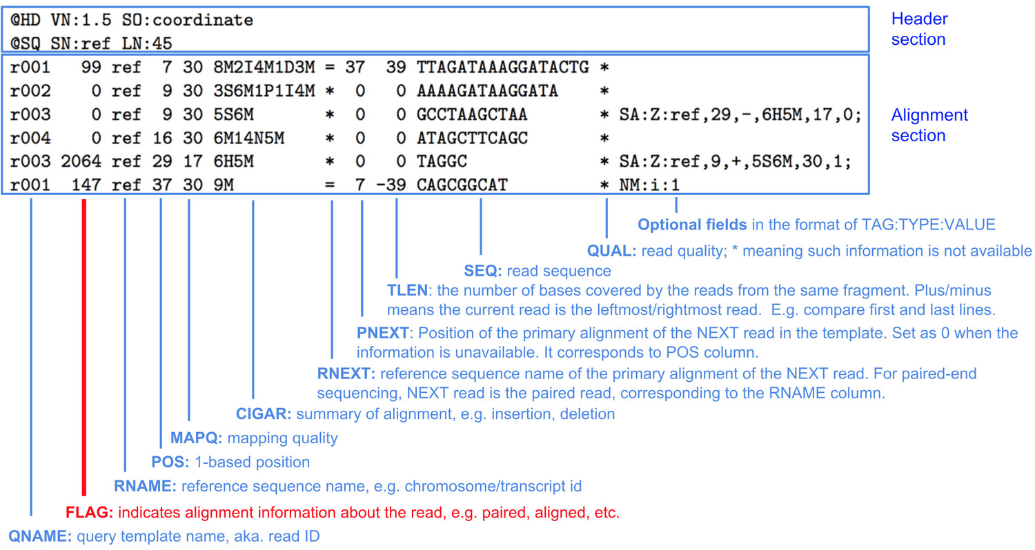
The standard format for aligned sequence data is SAM (Sequence Alignment Map).
SAM files have a header that contains information on alignment and contigs used, and the aligned reads:

But because SAM files can be large, they are usually stored in the compressed version of them, BAM files.
Multiple algorithms have been developed to align long reads to a genome of reference. Some examples are:
- Graphmap: http://github.com/isovic/graphmap
- bwa mem -x l ont2d: http://github.com/lh3/bwa
- LAST: http://last.cbrc.jp
- NGMLR: http://github.com/philres/ngmlr
- minimap2: http://github.com/lh3/minimap2
Here we will use NGMLR. First we will map the reads to the genome of reference (GRCh37), and convert the SAM output to BAM format.
ngmlr -r ~/Course_Materials/human_g1k_v37.fasta.gz -q ../data/fastq/NA12878.ROI.fastq -o alignment/NA12878.ROI.sam
samtools view alignment/NA12878.ROI.sam -O BAM -o alignment/NA12878.ROI.bam
Then, we will sort it by mapping coordinate and save it as BAM.
samtools sort alignment/NA12878.ROI.bam > alignment/NA12878.ROI.sort.bam
Finally we will index the BAM file to run samtools subtools later.
samtools index alignment/NA12878.ROI.sort.bam
To visualise the BAM file:
samtools view alignment/NA12878.ROI.sort.bam | less -S
Alignment QC
As a first QC, we can run samtools stats:
samtools stats alignment/NA12878.ROI.sort.bam > stats/stats.txt
head -n40 stats/stats.txt
- How many reads were mapped?
- Which was the average length of the reads? And the maximum read length?
Now we will get the coverage per base using samtools depth.
samtools depth alignment/NA12878.ROI.sort.bam > stats/coverage.txt
And look at the coverage distribution in R. For that, you can start R from the command-line:
R
and then, type the following:
library(ggplot2)
coverage <-  read.table("stats/coverage.txt", header=FALSE, col.names = c("chrom", "pos", "cov"))
cov_percent <- data.frame(  "cov" = seq(1,max(coverage$cov))
                          , "percent" = sapply(seq(1,max(coverage$cov)), function(x) nrow(coverage[coverage$cov >= x,])/nrow(coverage)))
p <- ggplot(cov_percent, aes(x = cov, y = percent)) +
     geom_line() +
     scale_x_continuous(breaks=seq(0,max(coverage$cov), 10)) +
     xlab("Coverage") +
     ylab("Percentage of bases")
p
You can also add a vertical line to the previous plot intercepting the median coverage:
p + geom_vline(xintercept=median(coverage$cov), colour = "red")
However, this is a very specific subset, and is not a representation of the coverage of NA12878’s genome. If you want to compare this with the coverage distribution across the whole genome, you can do the same steps but for the NA12878.
Variant calling
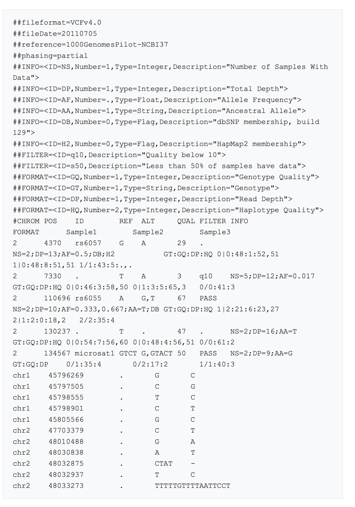
Variants are called and stored in VCF format. This contains a header, and then data lines each containing information about a position in the genome.

Currently, there are different algorithms for calling SVs from long-read sequencing data, including:
Since we used NGMLR for the alignment, now we will use sniffles for calling structural variants.
sniffles -m alignment/NA12878.ROI.sort.bam -v variant_calling/NA12878.ROI.vcf
If you want to look at high quality SVs, you can change the -s parameter to 20, where s is the minimum number of reads that support a SV (by default is 10).
sniffles -m alignment/NA12878.ROI.sort.bam -v variant_calling/NA12878.ROI.s20.vcf -s 20
The information that is provided in sniffles’s output can be found in: http://github.com/fritzsedlazeck/Sniffles/wiki/Output
To know how many SVs have been called, we will run:
bcftools view -H variant_calling/NA12878.ROI.vcf | wc -l
Finally, you can convert the VCF to a tab format:
../scripts/vcf2tab.py variant_calling/NA12878.ROI.vcf
and inspect the deletions in IGV.
- How many deletions are real?
- How many SVs breakpoint junctions are within repetitive sequences?
- For that, you would need to load Repeatmasker from server (File > Load from server > Annotations > Variation and Repeats > Repeat Masker)